Robotic scrub nurse to anticipate surgical instruments based on real-time laparoscopic video analysis

Prerequisites

Contextual execution of robotic autonomous actions using ML methods requires data along a surgical intervention³⁷. The data can be obtained from different sensory modalities, such as vision, audio, physiological or device signals. During laparoscopic procedures, endoscopic video data is the crucial data source as it provides a view of the surgical field. Current research focuses mainly on identifying surgical phases^38,39,40,41 and detecting or segmenting surgical tools^{42,43,44,45,46,47} based on laparoscopic videos⁴⁸. Various data sets^38,44,49,50 are available for this purpose, ranging from binary annotations to segmentation masks.

In our setup, we also use the laparoscopic video signal as input for our RSN system, providing the basis for predicting the next required instrument. The RSN is located in the sterile area next to the operating table as shown in Fig. 2 and performs the tasks of a human scrub nurse. The surgeon has access to the patient’s intra-abdominal area through a left and right working trocar. Thus, the surgeon inserts the laparoscopic instruments into the abdominal cavity, where they are visible in the endoscopic video. The first assistant is usually responsible for guiding the endoscope.

Task formulation

Since unimodal data sets only contain the instrument presence within laparoscopic videos, we must calculate the robotic prediction time of the next required instrument retroactively from the time t₀ another instrument is last used before it is changed. We set the prediction time t_pred = t₀ − δ so that the prediction must take place at least δ seconds before the last instrument is extracted to ensure that the robotic assistance has enough time to prepare the next required instrument. With a certain acceptable threshold, we can identify a prediction window w_p (t_pred ± τ), in which the instrument change should be correctly predicted. In addition, the prediction window is shifted (σ) to overlap the point of instrument extraction, allowing the model to learn on disappearance of the instrument from the endoscopic image. Considering the substantial delay the robotic arm introduces due to its slow movement pattern, a resting window w_r must be established, punishing premature movement which would prevent or at least delay the correct movement in the prediction window. We also introduce a disregard window w_d, representing periods between prediction and resting windows in which no prediction should take place.

In contrast to previous attempts at surgical instrument anticipation^33,34,35, we formulate the instrument anticipation task as a classification problem. Given a frame i from a video at time t_i, we extract the visual feature vector V, the detection feature vector D, and the segmentation feature vector S. Based on this observed sequence V_i, D_i, S_i, our model attempts to classify the anticipative status y_λ(i, α) of the next required instrument λ depending on the surgery phase α in the prediction window, which triggers the robotic handover of the predicted instrument to the surgeon. During the resting window, the model should set the predictive status to idle y₀(i, α) to prevent the robot from making any movement. This process is illustrated in Fig. 3. Our model predicts the next required instrument for each working trocar of the surgeon separately, enabling enhanced context sensitivity of the surgery.

For δ = 3 s, τ = 3 s and σ = 1 s the prediction window ranges from t₀ − 6 s to t₀ + 1 s. In the prediction window, the next required instrument is predicted. Subsequently, the predicted instrument is picked up by the RSN and transferred to the surgeon, who inserts it into the corresponding working trocar. At time t₀, the instrument disappears from the laparoscopic video. A resting window precedes each prediction window to prevent possible false predictions and premature movements of the robot.

Network architecture

The proposed model consists of ResNET50⁵¹ and YOLOv8⁵² for visual feature extraction followed by a Long-Term Context (LTContext) architecture⁵³ and a self-designed informed model. The full network architecture is visualized in Fig. 4.

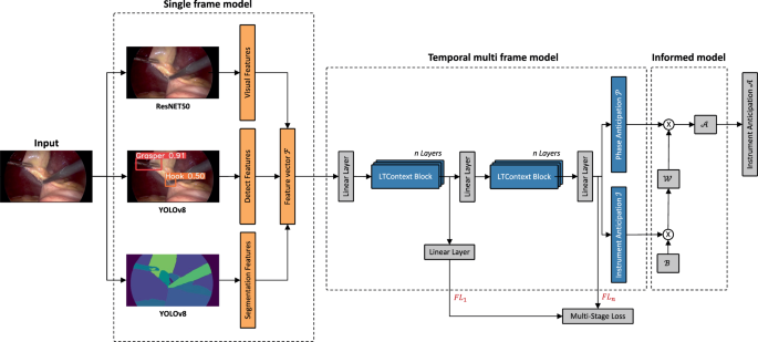
The architecture is composed of three feature extractor backbones, whose outputs are concatenated in the feature vector F. The feature vector is refined by a temporal multi frame model consisting of multiple stages of transformer-based LTContext blocks for anticipation of the next required instrument and the corresponding surgical phase. A subsequent informed model validates the prediction of the instrument using a phase compatibility matrix and adjusts uncertain predictions. The focal loss is calculated after each stage and aggregated for the joint training of the model.

Due to its success in prior studies³⁹, a ResNET50 was trained frame-wise without temporal context as a feature extractor from the videos on laparoscopic instrument, phase and action detection. The results of the feature extraction are the image features V ∈ R²⁰⁴⁸ per image and the corresponding class probabilities \(p(V)\in [0,1]^c_v\) with c_v as the number of classes. Using c_v = 34 classes (12 instruments, 11 phases and 11 actions) concatenated with the image features yields the visual feature vector V ∈ R²⁰⁸².

We trained a YOLOv8 network to recognize the laparoscopic instrument class and the spatial coordinates in terms of bounding boxes, resembling an instrument interaction module³⁴ to model the surgeons’ intention during surgery. Instead of encoding the geometric relation between the grasper and other instruments, we concatenated the instrument class c_i, the bounding boxes (x_i, y_i, w_i, h_i), and the bounding box size s_i = w_i ⋅ h_i of each detected instrument, resulting in the detection feature vector \(D\in R^c_i\times 6\).

To model the instrument’s nearby anatomical structure, we trained another YOLOv8 network on organ and instrument tip and shaft segmentation. From the resulting segmentation masks, we calculated different image shape measurements such as eccentricity, extent, orientation, perimeter, and solidity for each detected organ, instrument tip or shaft class c_s. In addition, we concatenated the number of class areas, the proportion of a frame in the area, and the relative x and y position of an area with the image shape measurements, yielding the segmentation feature vector \(S\in R^c_s\times 9\).

The feature vectors V, D, and S are concatenated and sent into the temporal multi frame model for the temporal phase and instrument anticipation task. The LTContext model consists of several stages S_i…M to refine the output of the first stage S₁. In contrast to ref. ⁵⁴, we modified the model to be fully causal, allowing for intraoperative online deployment. After each stage S_1…M we use the focal loss⁵⁵ (FL) to accurately train our model on the rarely occurring instrument changes. Moreover, we weight the focal loss with the scaling function shown in Eq. (1) to focus on predictions at the beginning of the prediction window, which results in well-timed triggering of the robotic motion. The variables β and μ are hyperparameters. The degree of temporal scaling is adjustable by β, whereby μ defines the weighting of the disregard window w_d.

Multiplying the scaling function with the adjusted focal loss for multiclass classification and adding the losses of the individual stages M yields the overall loss function in Eq. (2). For both the resting and the prediction window, we set the focusing parameter γ = 2, while for the disregard window we set γ = 1.

To make the anticipation of an instrument even more reliable, we incorporate prior surgical knowledge by an informed model using an instrument phase compatibility matrix B. This binary matrix describes the natural usage of laparoscopic instruments in the respective phases of a surgery. By performing matrix multiplication with the instrument anticipation matrix I and instrument phase compatibility matrix B, we compute the weighted instrument matrix W = I × B. The resulting weighted instrument matrix W assigns weights to each instrument based on its compatibility with other instruments, as determined by the binary relationships encoded in B. After normalizing the phase anticipation matrix P and the weighted instrument matrix W, we again perform matrix multiplication to obtain our final normalized instrument anticipation matrix \(A^\prime =P^\prime \times W^\prime\).

Data sets

We created two non-publicly available data sets to train the RSN with real-world data. We recorded laparoscopic videos of 12 cholecystectomies at the University Hospital rechts der Isar with a resolution of 1920 × 1080 pixels at 50 frames per second (fps). The 12 cholecystectomies were semantically annotated at 1 fps by medical experts with the annotation tool CVAT⁵⁶. All videos provide pixel-wise annotation of laparoscopic instruments, while one video also includes pixel-wise annotation of the anatomical structure. This data set was used for learning the feature vectors D and S.

The second data set, which we also recorded at the University Hospital rechts der Isar, includes 50 laparoscopic videos with a resolution of 1920 × 1080 pixels recorded at 25 fps or 50 fps. The data set contains the annotation of 11 phases, 12 instruments, and 11 actions. In addition, it provides information about the working trocar occupation of the laparoscopic instruments. The phases, instruments, actions, and trocar occupation were annotated by medical experts with the annotation tool ELAN⁵⁷. The 50 videos were randomly split into training (68%), validation (16%), and test (16%) sets and used for learning both the feature vector V and the temporal multi frame model. The videos were sub-sampled to 1fps and resized to a spatial resolution of 224 × 224 pixels to reduce computational costs.

The data were collected with ethical approval and written informed consent from the participants. Approval was granted by the Ethics Committee of the University Hospital rechts der Isar (No. 337/21 S). This study was performed in line with the principles of the Declaration of Helsinki. The authors also affirm that they have received written informed consent from all individuals for the publication of the images contained in this manuscript.

Model training and deployment

The YOLOv8 feature extractors were trained on the first data set while the ResNET50 was trained on the second data set. The temporal model was also trained on the second data set using a hyperparameter sweep. The best results for the task of surgical instrument anticipation were achieved for the number of stages S = 1 and layers n = 8 using the Adam optimizer with an initial learning rate of 5e − 5 for 550 epochs. The warm-up amounted to 70 epochs. We provide the test results of the model that performed best on the validation set. The batch size is identical to the length of each video. The model was implemented in PyTorch and trained on three NVIDIA RTX A6000s. For intraoperative online deployment, we built an inference pipeline using NVIDIA Clara Holoscan. The model outputs are transferred from a NVIDIA AGX development kit to the robot via the robot operating system (ROS).

Evaluation metrics

To comprehensively measure the results of the predictions, we consider each resting window followed by a prediction window as one sequence. We set the label of the sequence equal to the ground truth of the prediction window. For each sequence, we check whether the first prediction \(\haty(i,\alpha )\, \ne \, y_0\) matches the corresponding label y(i, α) and track the position of the occurrence of the prediction. For comparing \(\haty(i,\alpha )\) against y(i, α), the confusion matrix for the prediction window \(C_w_p\) and the resting window \(C_w_r\) are computed. By embedding \(C_w_r\) in \(C_w_p+w_r\), we can evaluate the performance of the ML system in a differentiated way and at the same time evaluate how well the integration of the robotic system can be realized (see Fig. 5). Based on the confusion matrix we deploy four different metrics suitable for classification tasks, namely precision, recall, accuracy and F1 score⁵⁸:

The evaluation metrics are computed class-wise, for each instrument and working trocar individually, and then averaged over all videos (operations) in the test set, yielding the weighted-averaged precision (wAP), recall (wAR), accuracy (wAA) and F1 score (wAF1). The weighted-averaged metrics are calculated by taking the mean of all per-class scores while considering each class’s support, whereby the support refers to the number of actual occurrences of the class in the test data set. In Supplementary Table 3 and Supplementary Figs. 11 and 13, we also provide the macro average metrics⁵⁹ per class as well as a multiclass confusion matrix for each working trocar separately. In this context, we neglect predictions in the disregard window w_d as these predictions do not harm the surgical workflow but would pose unnecessary robotic movements.

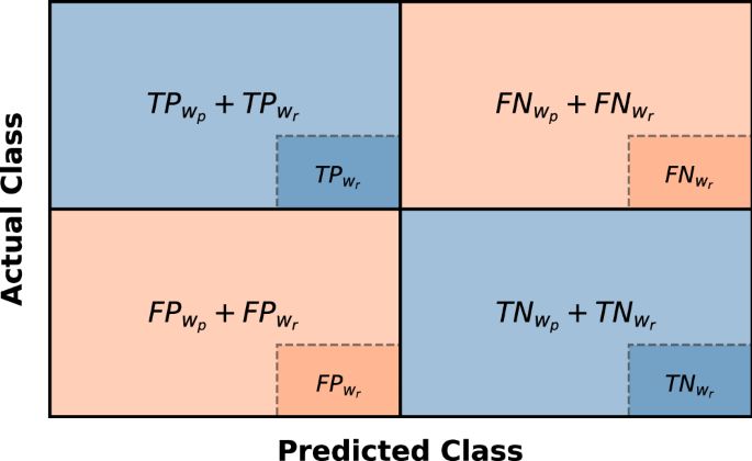
Confusion matrix of the resting window \(C_w_r:= \TP_w_r,FP_w_r,FN_w_r,TN_w_r\\) embedded in the confusion matrix of the prediction window \(C_w_p:= \TP_w_p,FP_w_p,FN_w_p,TN_w_p\\). The metrics are calculated based on both confusion matrices.

Statistics and reproducibility

The model performance was assessed using the metrics described such as weighted-averaged precision, recall, accuracy and F1 score. Hyperparameter tuning was conducted using Bayesian search. The data set for learning the instrument anticipation task consisted of 50 samples, which were randomly split into training and testing sets. The training set contained 34 samples, while the testing set contained 8 samples. A validation set of 8 samples was used for hyperparameter tuning. The temporal multi frame model was trained 10 times using different random seeds to initialize the model parameters assessing stability and reliability of the model performance.

Reporting summary

Further information on research design is available in the Nature Portfolio Reporting Summary linked to this article.